GridSight

Understanding Candle Dynamics: The Power of 3

Every price candle tells a story through its four key reference points:

• Open: The starting price of the time period
• High: The maximum price reached during the period
• Low: The minimum price reached during the period
• Close: The final price at period end

What makes these points powerful is their sequence. This sequence is known as the "Power of 3" because it reveals three distinct market phases:

1. Accumulation: Initial price movement from open
2. Manipulation: Creation of the high or low (first extreme)
3. Distribution: The primary directional move toward close

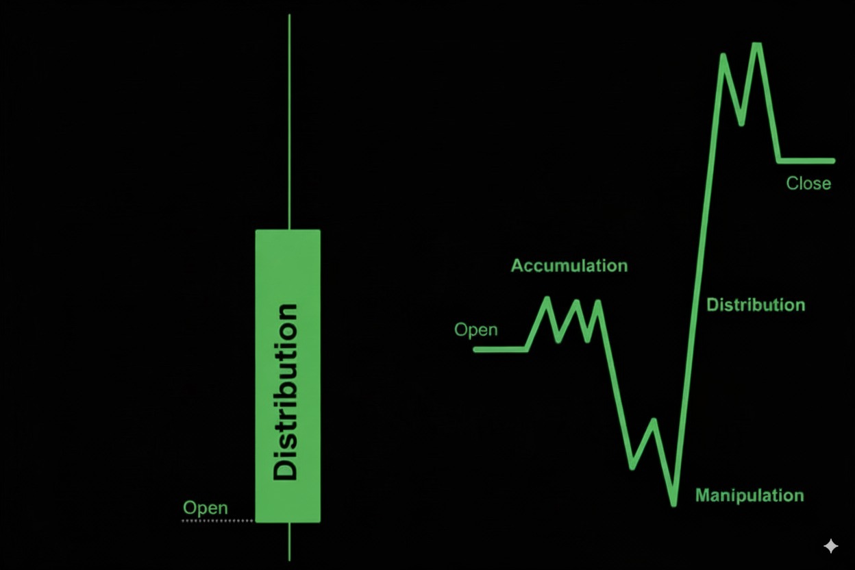
For bullish candles, the typical sequence is open → low → high → close, while bearish candles follow open → high → low → close. This pattern isn't random—it represents how institutional order flow typically moves through a time period.

The critical insight: Profitable trades align with this natural order flow. By entering after the first extreme forms (the low in bullish candles, the high in bearish candles), we can capture the distribution phase—the most substantial and predictable portion of the move.

Price Dimension: Premium and Discount Zones

To identify where these extremes are likely to form, we analyze price deviations from the opening price:

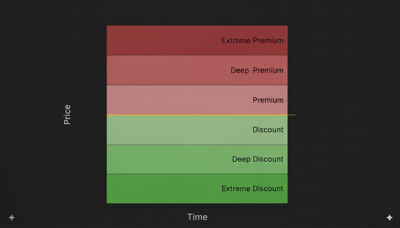
Discount Zones (Bullish Bias)

When our bias is bullish, we focus on discount zones—areas below the opening price to look for the first extreme to form (LOW):

• Shallow Discount: Closer to opening price, higher probability of low formation but smaller reward potential
• Deep Discount: Further from opening price, lower probability of low formation but larger reward potential

Premium Zones (Bearish Bias)

Conversely, when our bias is bearish, we focus on premium zones—areas above the opening price to look for the first extreme to form (HIGH):

• Shallow Premium: Closer to opening price, higher probability of high formation but smaller reward potential
• Deep Premium: Further from opening price, lower probability of high formation but larger reward potential

This logic can be extended for the second extreme as well.

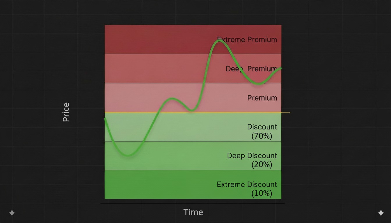
Probability Framework

The mathematical framework for analyzing these zones uses conditional probability: Lets assume our bias is bullish

P(X|Y) where:

• Y = The candle will close bullish (bullish bias)
• X = The low will form in a specific price range bucket [a-b]% from the open
• P(X|Y) = The probability of the low forming in a specific price range bucket [a-b]% from the open given that the candle will close bullish (bullish bias)

In the figure below we visualize this idea with sample probabilities

Conversely we can look at the second extreme which in this case would be the high of the candle if our bias is bullish

P(Z|Y) where:

• Y = The candle will close bullish (bullish bias)
• Z = The high will form in a specific price range bucket [a-b]% from the open
• P(Z|Y) = The probability of the high forming in a specific price range bucket [a-b]% from the open given that the candle will close bullish (bullish bias)

This simple framework is quite useful and widely available in the community, however we can take things much further by incorporating time alongside price.

Time Dimension: Evolution of Probability

The innovation of GridSight is incorporating the temporal dimension. As a candle progresses, the range of possible outcomes narrows. There are also statistical properties of the time dimension that we can take advantage of.

Dynamic Probability Assessment

As time elapses within a candle period:

• Early Stage (0-25%): Maximum uncertainty, all scenarios remain possible, first extreme forms
• Mid Stage (25-75%): Partial structure formation, some paths eliminated, main distrbution phase forms
• Late Stage (75-100%): Limited remaining volatility, high predictability, second extreme forms

GridSight continuously updates its probability model as new price information becomes available:

• Prior Probability: Initial statistical assessment based on historical patterns
• New Information: Real-time price action during candle formation
• Posterior Probability: Updated assessment that incorporates both prior knowledge and new data

The Time-Price Matrix: Integrating Price and Time

The core of GridSight is a dynamic two-dimensional probability matrix that maps the likelihood of extreme formation across both price and time dimensions:

• Vertical Axis: Price deviation from opening (premium/discount percentage)
• Horizontal Axis: Time elapsed in candle (percentage of completion)

Practical Applications

Lets follow a simple example to understand how GridSight works.

Visualizing the Probability Grid

The GridSight matrix provides a visual representation of probabilities across both time and price dimensions:

• Red Cells: In a bullish bias scenario, represent the probability of the low (first extreme) forming in that specific time-price coordinate
• Green Cells: Represent the probability of the high (second extreme in bullish bias) forming in that specific time-price coordinate

As the candle forms and time progresses, these probabilities dynamically update. Early in the candle, probabilities are more evenly distributed, but as time elapses and price moves, certain cells gain higher probability values while others approach zero.

The figure below shows a sample grid for a bullish bias scenario right at the start of the candle

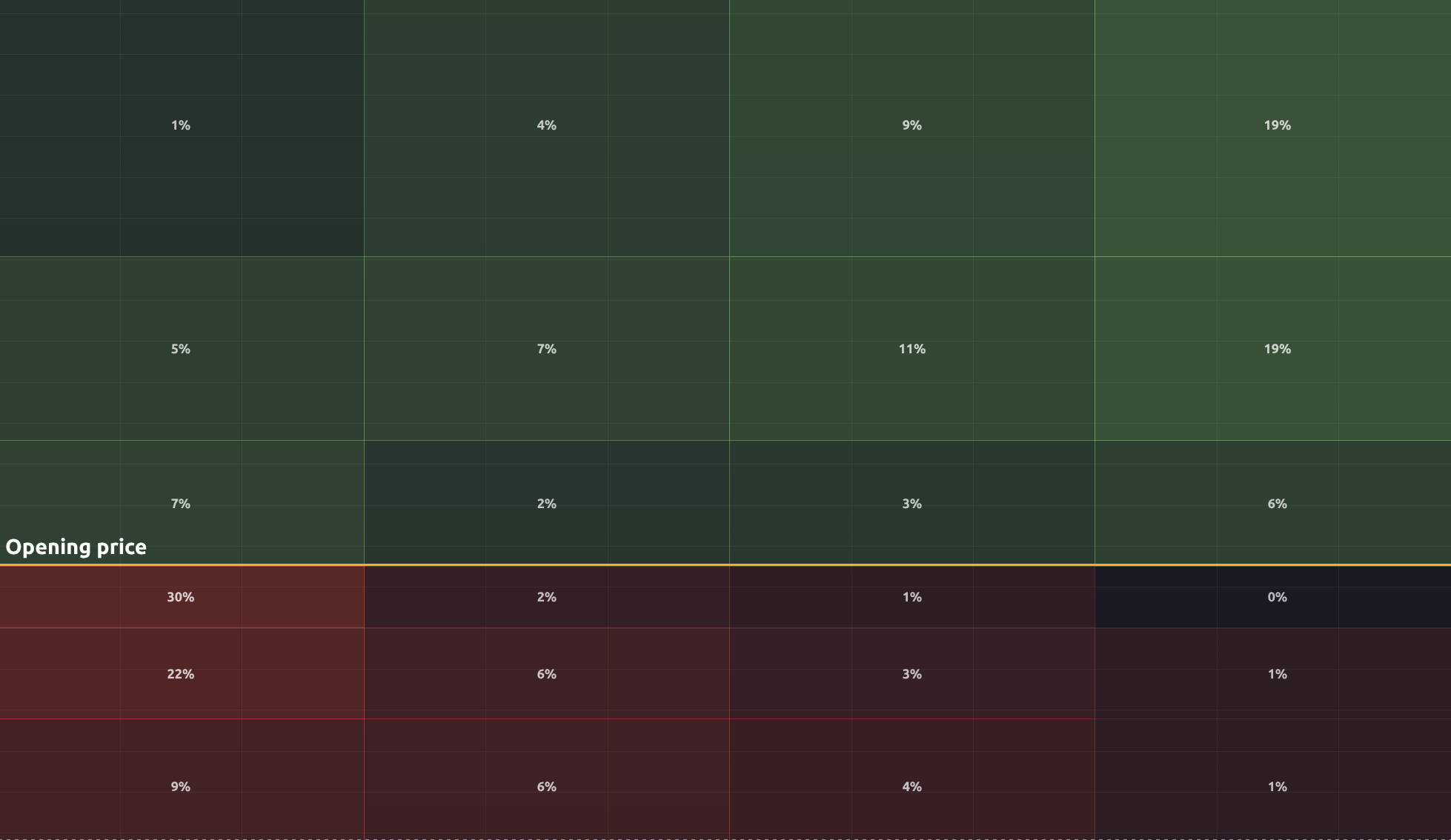
Determining Directional Bias

One of the most challenging aspects of trading is establishing a directional bias. GridSight requires an initial bias input, but also provides a systematic approach when no clear bias exists:

1. First Column Analysis: The first extreme typically forms in the early stages of a candle (first column of the grid)
2. Range Breakout Method: When price trades beyond the initial range established in the first column:
   • If price exceeds the first column's high → Assume bullish bias (low has likely formed)
   • If price drops below the first column's low → Assume bearish bias (high has likely formed)

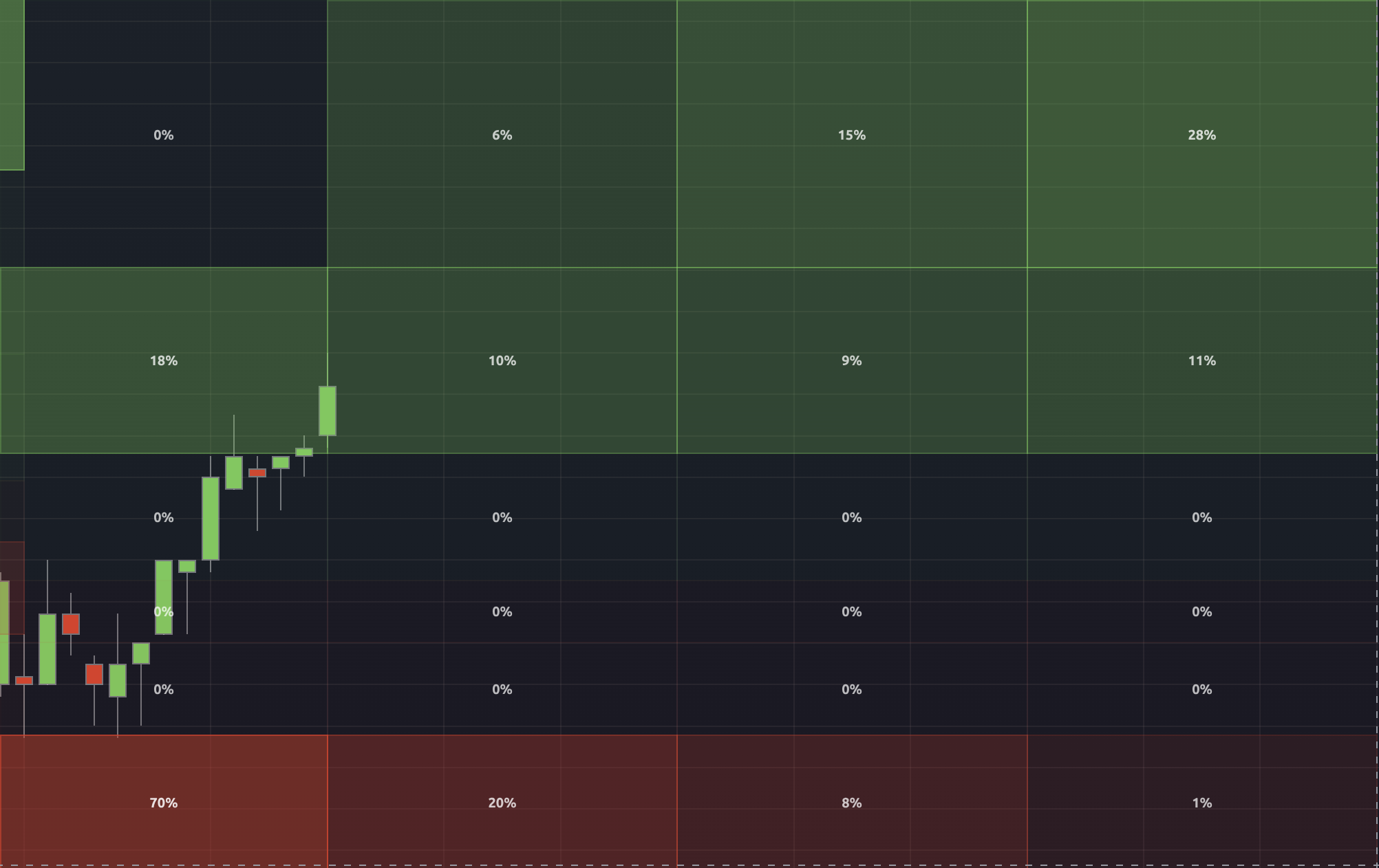
This method allows traders to adapt to the emerging Power of 3 structure as it develops, rather than requiring a predetermined bias. In our example we notice that there is a 61% chance of the low forming in the first column, once price breaks above the first column high we can assume the bias is bullish.

The probabilities update once we hit the first column of the grid, 25% of the candle is complete. Note the high and low of this range.

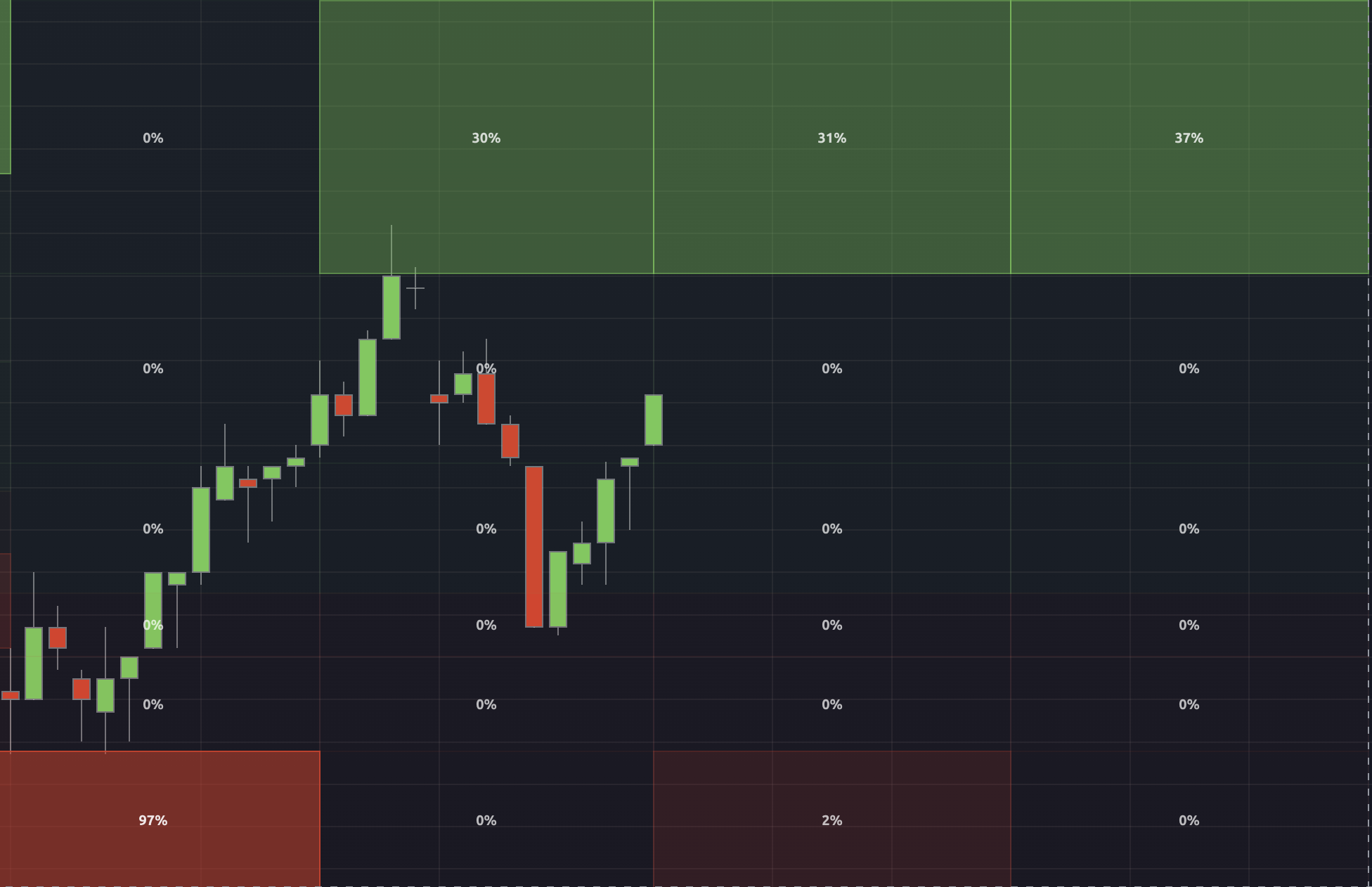
We've broken above the first column high, so we can assume the bias is bullish. Now we can notice that there is a 68% chance of making a new high, and our low is locked in at 97% probability. This sets up the context to look for longs.

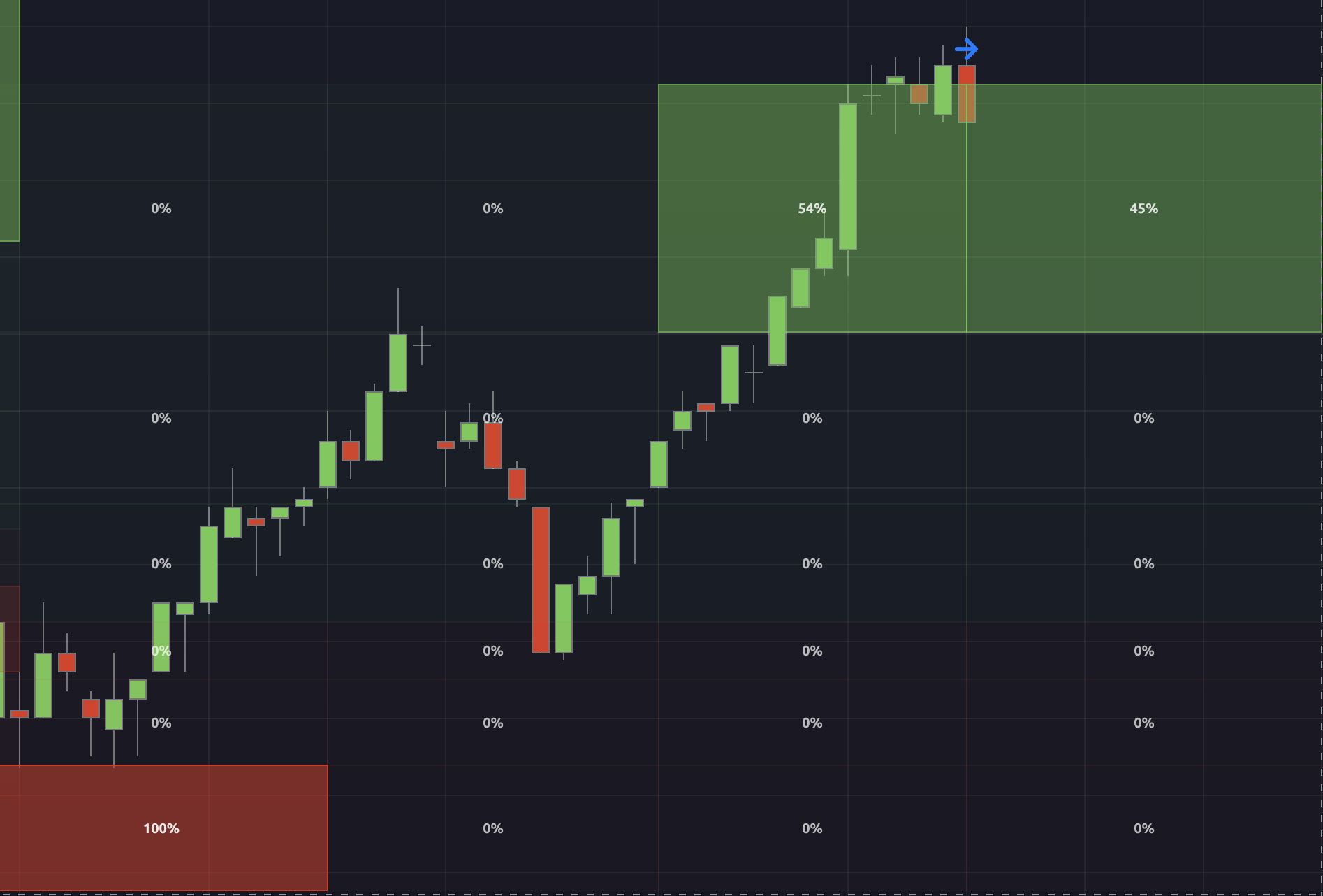
We push higher to create a new high

Optimizing Trade Execution

Entry Timing

GridSight provides statistical guidance for optimal entry points:

1. First Extreme Confirmation: Wait for the first extreme to form (identified by high-probability cells)
2. Direction Alignment: Enter in the direction of the anticipated distribution phase
3. Probability Threshold: Consider entries when the probability of the first extreme having formed exceeds a predetermined threshold (e.g., 75%)

Exit Strategy

The second extreme statistics inform realistic profit targets:

1. Second Extreme Projection: Use the probability distribution of the second extreme to set profit targets
2. Time-Based Adjustment: Adjust targets based on remaining candle time
3. Probability Gradient: Consider partial exits at different probability thresholds

Risk Management

The probability matrix provides a statistical foundation for stop loss placement:

1. Low-Probability Zones: Place initial stops in areas with minimal statistical likelihood of price reaching
2. Dynamic Adjustment: Trail stops more aggressively as the first extreme becomes more clearly defined

Multi-Timeframe Analysis

GridSight's effectiveness increases significantly when applied across multiple timeframes:

1. Probability Stacking: Identify setups where high-probability zones align across different timeframes
2. Nested Structure: Use higher timeframe bias to inform lower timeframe execution
3. Confluence Points: Focus on price levels where multiple timeframe probability peaks converge

By stacking GridSight analysis across timeframes, traders can identify situations where statistical edges compound, creating particularly high-probability trading opportunities.

This systematic approach transforms the subjective art of trading into a more objective, probability-based discipline that aligns with the algorithmic price movement.

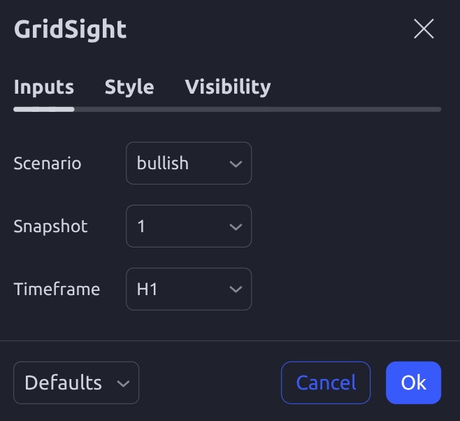
Settings

The settings are as follows

Scenario: Bullish or Bearish. The bias assumption that the candle will be up or down close

Timeframe: D, H4, H1. The timeframe to apply the grid to

Snapshot: 1,2,3,4, or latest. Snapshot can be used to backtest the grid at different stages of the candle, latest will always get you the most recent data